Drug Release Kinetics Models: Zero Order, First Order, Higuchi, Korsmeyer-Peppas

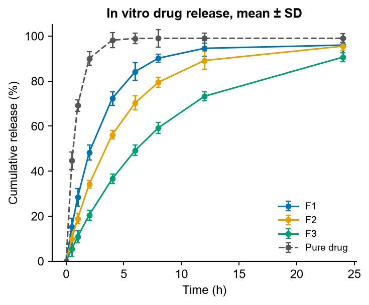
In vitro release data are usually fitted to several kinetic models, and the model with the highest R² (and a sensible mechanism) is reported. These are the models used most in pharmacy theses and papers.

Zero order

Q_t = Q₀ + K₀t. Plot cumulative % released against time. The drug is released at a constant rate, as in ideal controlled-release systems such as some osmotic tablets and transdermal patches.

First order

log C = log C₀ − Kt / 2.303. Plot log % drug remaining against time. The rate depends on how much drug is left, typical of many porous matrices with water-soluble drugs.

Higuchi

Q = K_H √t. Plot cumulative % released against the square root of time. A straight line suggests diffusion-controlled release from a matrix.

Korsmeyer-Peppas

M_t/M_∞ = K tⁿ. Plot log cumulative % released against log time, using only the first 60% of release. The slope n hints at the mechanism. For a thin film: n ≤ 0.5 Fickian diffusion, 0.5 < n < 1 anomalous (non-Fickian) transport, n = 1 case II (relaxation) transport. For cylinders the limits are about 0.45 and 0.89, and for spheres about 0.43 and 0.85.

Hixson-Crowell

Q₀^1/3 − Q_t^1/3 = K_HCt. Used when the particle surface area and size change as the drug dissolves.

Plotting the release profile

Show mean ± SD (n ≥ 3) at each time point, with formulations as separate lines.
Include the pure drug as a reference.
Give the release medium, temperature and method (for example dialysis bag, pH 7.4, 37 °C) in the legend.

Upload your release data to the Drug Release Profile tool for a journal-style plot.

Make your figure nowDescribe it or upload a sketch. Free to start. Open SciFigures